LED Strip Calculations#
The idea is to construct a spiral (Archimedean spiral or others) around a right-cone simulating a Christmas tree. We want to model the situation and understand how many lights or how long the strip(s) should be to wrap the proper amount of loops around the tree. This blog will establish the basic model and mathematics. This article will walk you through the mathematical derivation and the calculations. The derivations are for completeness. An understanding of the process is not required to use the results.
LED Design#
We want to construct a set of methods and equations that can describe an LED strip arranged in a spiral around a right-circular cone with base radius \(r\) and height, \(h\).

Figure 1 - Right-Cone.#

Figure 2 - Right-Cone - Top View.#

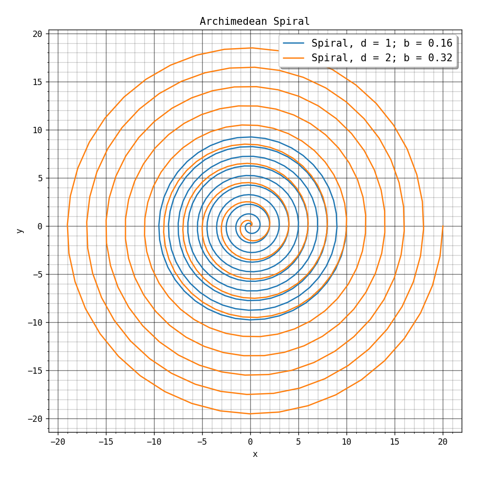
Figure 3 - Sprials around the cone.#
Archimedian Spiral#
The Archimedean spiral is the simplest of the spirals. It is defined, in polar coordinates, by:
Where:
\(r(\theta)\) - The distance to a point on the curve defined by \(\theta\)
\(\theta\) - An angle
\(b\) - A constant defining the distance between successive intersection points between the curve and the axis
\(p\) - A constant, the initial radius of the curve, the starting point
Note
The Archimedean spiral is also an arithmetic spiral.
Note
The distance between two successive turns is \(d = 2 \pi b\). In other words, the distances of intersection points along a line through the origin and the spiral are the same.
Note
For this article we are going to assume \(p = 0\).
Parametric Form#
The general parametric equations are:
Convert the polar equation (1) to parametric form:
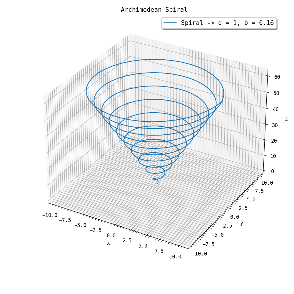
3D#
We can extend the parametric system to three dimensions:
Where:
\(z_0\) - The initial starting position of the spiral
\(m\) - The slope of the cone with respect to the
XYplane
Note
We’ll assume that \(\theta \ge 0\)
Re-Worked Model#
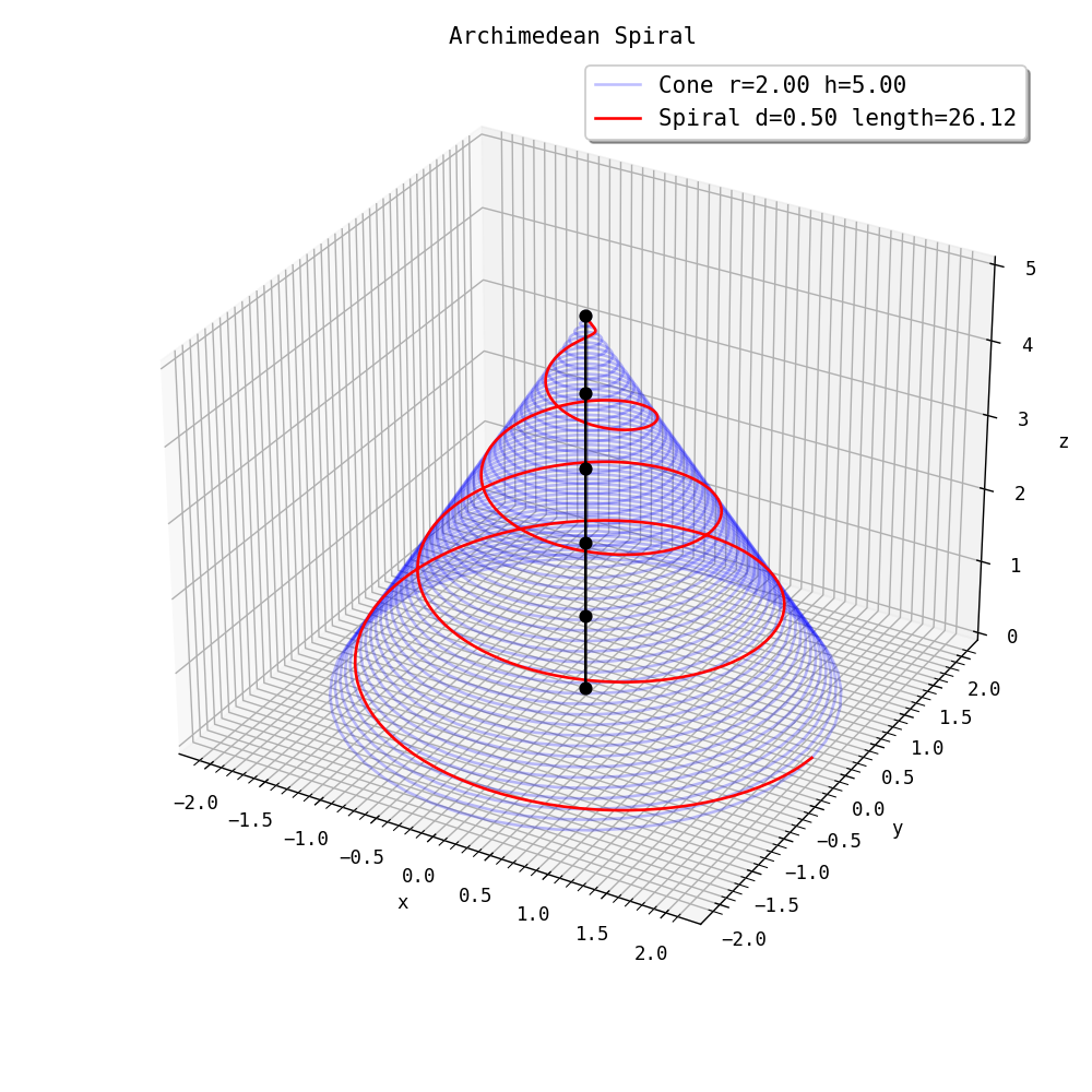
I want the spiral to look like a tree. The spiral opens upwards and looks like an inverted tree given positive angles. I want the spiral to open downwards, starting from the top of the cone to the base. It should also end with the radius that matches the radius of the cone itself. Let’s re-work the model. We will use the same set of equations as defined in (4). We will use negative angles and starting from \(z_0 = h\) to achieve the effect:
We also want to stop the spiral when:
If we know \(b\) and \(r\), we can solve for the stop angle, \(\theta\):
We also need to solve for \(m\) to determine the proper slope of the cone so the spiral fits within our constraints.
In our case, \(z(\theta) = 0\) and \(z_0 = h\), simplifying (7) yields:

Cone Radius (r) = 2.0000
Cone Height (h) = 5.0000
Conical Spirals - Arc Length#
In the previous section, 0 - conical spirals.ipynb, we developed the model to trace the Archimedean spiral around the cone. In this section, we explore the derivation of the equations to calculate the arc length of the spiral (Archimedean spiral). In practical terms, if we use LED strips to create a spiral around the cone, we can determine the required LED strip length to get the job done.
Note
The full Jupyter notebooks can be found in this repository. This section can be found here.
Arc Length of a Curve in Polar Coordinates#
Now that we can plot the spiral, how long is it? Essentially, we want to determine the length of the vector function:
Writing the vector function in parametric form:
In 3 Dimensions, the length of the curve, \( \vec r \left(t \right)\) on the interval \(m_1 \le t \le m_2\) is:
Note
In the notebook, 0 - conical spirals.ipynb, we represented the angle as \(\theta\). For this derivation, consider \(t = \theta\). We will continue to use \(t\) to represent the polar angle.
The parametric equations for the spiral are:
Where \(b\) and \(k\) are constants that control the shape and height of the spiral and \(t\) is the angle in radians controlling the number of loops.
Note
In the notebook, 0 - conical spirals.ipynb, we represented the shape of the cone with \(m\). For the rest of this document, consider \(k = m\), from this point forward.
Take the derivative of each equation:
Let’s rearrange things to make dealing with the polynomial and the radical easier:
Where:
Note
We made use of http://www.integral-calculator.com/ when solving the integrals.
Solve the integral and Substitute:
Simplify using:
Becomes:
Now Solving:
Apply reduction formula with \(n=3\):
Now Solving:
The solution is a standard integral. Plugin solved integrals:
Undo substitution:
Use:
Solution:
Note
Applying the limits will eliminate the constant…
Cone Radius (r) = 2.0000
Cone Height (h) = 5.0000
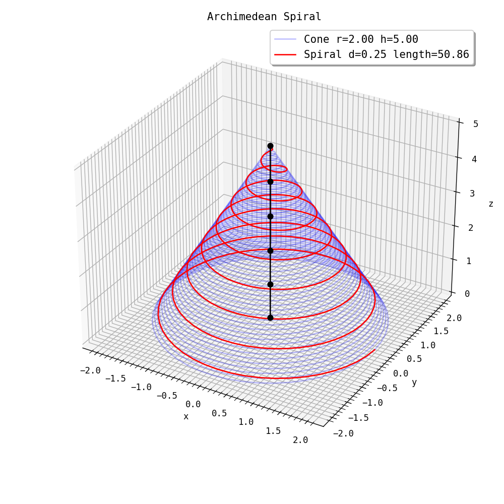
Conical Spirals - Supports#
Given a conical (Archimedean) spiral, calculate where we could place supports. We’ll assume they will be at integer intervals. If the height is 5 units, we’ll want support at 1, 2, 3 and 4. The way this works, we specify the support interval delta along with the cone’s height, Z, and it will calculate the locations and lengths of the support struts.
Note
The full Jupyter notebooks can be found in this repository. This section can be found here.
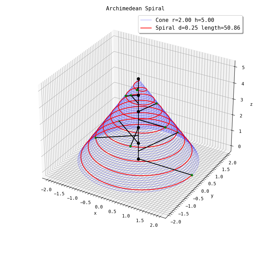
Support Points#
We want to find the points on the curve that intersect specific elevations between \(0\) and \(h\). Our current model:
The angles where the curve passes through specific elevations can be calculated with:
Essentially, we must calculate the particular angles that coincide with the heights of interest. In our case, we’ll simply use the integer values from \(0\) to \(h\).
Cone Radius (r) = 2.0000
Cone Height (h) = 5.0000
Strut Offset Height (Δh) = 0.5
------
Support Length (@ Z=0.0) = 2.00
Support Length (@ Z=0.5) = 1.80
Support Length (@ Z=1.0) = 1.60
Support Length (@ Z=1.5) = 1.40
Support Length (@ Z=2.0) = 1.20
Support Length (@ Z=2.5) = 1.00
Support Length (@ Z=3.0) = 0.80
Support Length (@ Z=3.5) = 0.60
Support Length (@ Z=4.0) = 0.40
Support Length (@ Z=4.5) = 0.20
The result is quite lovely! The support points are calculated at specific Z values, and the support strut lengths are calculated and plotted for those heights.
Future#
We could adjust the model to place supports at regular angles instead of regular elevations. For example, we could add supports at the regular angles (0, pi/2, pi, 3pi/2 + etc.). It would mean that we would trace the curve and put supports on the north, east, south and west sides. This might be easier to fabricate.
Fixed Arc Length#
The other sections will calculate the arc length of the spiral based on the cone width and height. This section will alter those parameters to fit a given arc length. Why do this? The primary use case is to fit a design to a specific LED strip length. For example, how big of a cone can you build using a 5m strip without cutting the strip or adding extra pieces.
Note
The full Jupyter notebooks can be found in this repository. This section can be found here.
Cone Radius (r) = 2.0000
Cone Height (h) = 5.0000
Find the Arc Length#
We want to determine the cone radius, height and loop spacing with a fixed spiral arc length. For example, we have a 5m strip, and we do not want to cut it. What radius, height, and loop spacing values will give us this fixed length? We’ll use the Scipy.Optimize modules to determine this.
Let’s construct a target function below, formulated in a compatible way with the optimize module.
def objective_fixed_length(x, L:float):
    """
    This method defines the objective function, the function we want to
    minimize. This particular instance will search for r, h and d, generating a
    particular arc length, L.

    # args

    x - 1-D array with shape (n,) of variables to solve for
        - x[0] - r - cone base radius
        - x[1] - h - cone height
        - x[2] - d - horizontal spacing between loops

    L - The arc length we are attempting to find.

    # NOTE

    From the Scipy.Optimization docs:

    The objective function to be minimized.

    fun(x, *args) -> float

    where x is an 1-D array with shape (n,) and args is a tuple of the
    fixed parameters needed to completely specify the function.

    We have to construct the target function using this method to accommodate
    the optimize module It uses an array to specify the target variables that
    we want to optimize and separate arguments for the constants we don't want
    to optimize.

    """

#     r, h, d = x
#     return np.abs(L - spiral_arc_length_range(r, h, d))

    return np.abs(L - spiral_arc_length_range(*x))
Let’s use the minimize method and see what we can do.
Note
We have to provide an initial guess for the other variables. The initial guess will affect the outcome. Most likely, there are many solutions to the problem. It is recommended to use values close to the dimensions of interest. The optimization uses the initial values to guide the process. In most cases, it will converge to the closest values.
arc_length = 5   # m
r_init = 1       # m
h_init = 3       # m
d_init = 0.5     # m

result = optimize.minimize(
    objective_fixed_length,
    (r_init, h_init, d_init),
    args=(arc_length,),
    method='Nelder-Mead',
    tol=1e-8,
)

print(result)
print('-------')

print('Optimal Values:')
print(f'r = {result.x[0]:.4f}')
print(f'h = {result.x[1]:.4f}')
print(f'd = {result.x[2]:.4f}')
 final_simplex: (array([[0.79863094, 3.15843977, 0.57331696],
       [0.79863094, 3.15843976, 0.57331696],
       [0.79863094, 3.15843976, 0.57331696],
       [0.79863094, 3.15843977, 0.57331696]]), array([1.97077732e-09, 3.20198268e-09, 3.69157505e-09, 5.59641045e-09]))
           fun: 1.9707773191157685e-09
       message: 'Optimization terminated successfully.'
          nfev: 165
           nit: 83
        status: 0
       success: True
             x: array([0.79863094, 3.15843977, 0.57331696])
-------
Optimal Values:
r = 0.7986
h = 3.1584
d = 0.5733
Let’s construct a method that can do the optimization and plot the results, plot_optimal:
def find_optimal(func, arc_length, r_init, h_init, d_init):
    """

    # args

    ax - matplotlib axis
    func - target function for optimization
    arc_length - the arc length we are interested in finding
    r_init - the initial guess for radius
    h_init - the initial guess for height
    d_init - the initial guess for loop horizontal spacing

    # Return

    A tuple containing the optimal radius, height and loop spacing (r, h, d)
    for the given arc length

    """

    result = optimize.minimize(
        func,
        (r_init, h_init, d_init),
        args=(arc_length,),
        method='Nelder-Mead',
        tol=1e-8,
    )

    return result.x
The code below demonstrates how to use the above function:
fig, ax = create_standard_figure(
    'Archimedean Spiral',
    'x',
    'y',
    'z',
    projection='3d',
    figsize=(8, 8),
    axes_rect=(0.1, 0.1, 0.85, 0.85),
)


arc_length = 5   # m
r_init = 2   # m
h_init = 3   # m
d_init = 0.5 # m

results = find_optimal(
    objective_fixed_length,
    arc_length,
    r_init,
    h_init,
    d_init,
)

plot_cone_and_spiral(ax, *results)

fig.show()
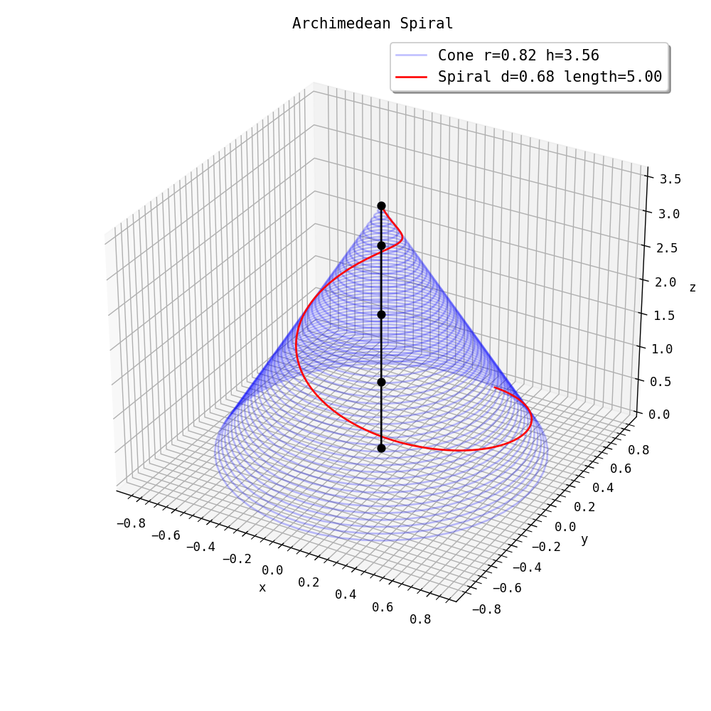
Cone Radius (r) = 0.8185
Cone Height (h) = 3.5565
From the above output, we can see that attempting to optimize for all variables at once leads to a lot of sub-optimal solutions. It might be better to simply hold more variables constant and vary only one at a time.
Optimal Cone - Fixed Loop Spacing - Vary Radius and Height#
Given that there are many solutions when we are able to vary the radius, height and loop width at the same time. What happens if we constrain the methods to only solve for radius and height? We’ll need to construct a new target function and a new optimal search routine.
# We have to construct the target function using this method to accommodate the
# optimize module It uses an array to specify the target variables that we want
# to optimize and separate arguments for the constants we don't want to
# optimize.
def target_function_rh(x, L, d):
    """
    This method defines the objective function, the function we want to
    minimize. This particular instance will search for r, h that generates a
    particular arc length, L with loop spacing, d.

    # args

    x - 1-D array with shape (n,) of variables to solve for
        - x[0] - r - cone base radius
        - x[1] - h - cone height

    L - The arc length we are attempting to find.
    d - The horizontal loop spacing we are interested in.

    # NOTE

    From the Scipy.Optimization docs:

    The objective function to be minimized.

    fun(x, *args) -> float

    where x is an 1-D array with shape (n,) and args is a tuple of the
    fixed parameters needed to completely specify the function.
    """

#     r, h, d = x
#     return np.abs(L - spiral_arc_length_range(r, h, d))

    return np.abs(L - spiral_arc_length_range(*x, d))
def find_optimal_rh(func, arc_length, d, r_init, h_init):
    """

    # args

    ax - matplotlib axis
    func - target function for optimization
    arc_length - the arc length we are interested in finding
    d - the initial guess for loop horizontal spacing
    r_init - the initial guess for radius
    h_init - the initial guess for height

    # Return

    A tuple containing the optimal radius, height and loop spacing (r, h, d) for
    the given arc length

    """

    result = optimize.minimize(
        func,
        (r_init, h_init),
        args=(arc_length, d),
        method='Nelder-Mead',
        tol=1e-8,
    )

    return result.x
fig, ax = create_standard_figure(
    'Archimedean Spiral',
    'x',
    'y',
    'z',
    projection='3d',
    figsize=(8, 8),
    axes_rect=(0.1, 0.1, 0.85, 0.85),
)


arc_length = 5   # m
d = 0.25 # m

r_init = 1   # m
h_init = 1   # m

results = find_optimal_rh(target_function_rh, arc_length, d, r_init, h_init)

plot_cone_and_spiral(ax, *results, d)

fig.show()
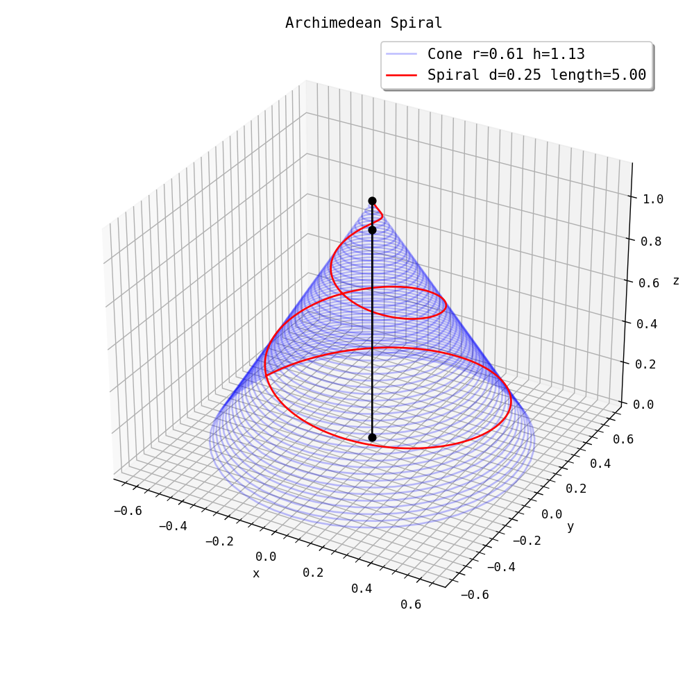
Cone Radius (r) = 0.6129
Cone Height (h) = 1.1321
By fixing the arc length and the d value, we can achieve better designs with less trial and error.
Optimal Cone - Fixed Loop Spacing and Radius - Vary Height#
In this case, we will keep the radius fixed and the loop spacing fixed, and we’ll simple vary the height.
# We have to construct the target function using this method to accommodate the
# optimize module It uses an array to specify the target variables that we want
# to optimize and separate arguments for the constants we don't want to
# optimize.
def target_function_h(x, L, r, d):
    """
    This method defines the objective function, the function we want to minimize.
    This particular instance will search for h that generates a particular
    arc length, L with loop spacing, d.

    # args

    x - 1-D array with shape (n,) of variables to solve for
        - x[0] - h - cone height

    L - The arc length we are attempting to find.
    r - The radius of the base of the cone
    d - The horizontal loop spacing we are interested in.

    # NOTE

    From the Scipy.Optimization docs:

    The objective function to be minimized.

    fun(x, *args) -> float

    where x is an 1-D array with shape (n,) and args is a tuple of the
    fixed parameters needed to completely specify the function.
    """

    return np.abs(L - spiral_arc_length_range(r, *x, d))
def find_optimal_h(func, arc_length, d, r, h_init):
    """

    # args

    ax - matplotlib axis
    func - target function for optimization
    arc_length - the arc length we are interested in finding
    d - the initial guess for loop horizontal spacing
    r - the initial guess for radius
    h_init - the initial guess for height


    # Return

    A tuple containing the optimal radius, height and loop spacing (r, h, d) for
    the given arc length

    """

    result = optimize.minimize(
        func,
        (h_init, ),
        args=(arc_length, r, d),
        method='Nelder-Mead',
        tol=1e-8,
    )

    return result.x
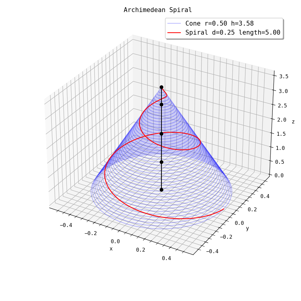
Cone Radius (r) = 0.5000
Cone Height (h) = 3.5841
LED Electrical Calculations#
Given an LED conical spiral of a given length, determine various electrical attributes about the setup. This could be multiple strips, including partials.
LED Details:
How many LED strips?
How many LEDs per strip? Per unit length?
How many amps per LED?
How many watts per LED?
LED strip voltage?
Questions?
Power requirements?
Power injection?
Power wire gauge?
Draw (amps) from mains?
The full Jupyter notebooks can be found in this repository. This section can be found here.
Formulae#
Where:
\(V\) - Voltage (Volts)
\(I\) - Amperage (Amps)
\(R\) - Resistance (Ohms)
Power#
Where:
\(P\) - Power (Watts)
\(V\) - Voltage (Volts)
\(I\) - Amperage (Amps)
\(R\) - Resistance (Ohms)
Example 1#
Using the strip from here as a reference. Strip details:
APA102
5m
60 LED/m
5V DC
18 Watt/m
import numpy as np
from scipy import optimize
length = 5                # m
LED_count = 60            # LED/m
watt_per_unit_length = 18 # watts per m
strip_voltage = 5 # volts

LED_total_count = LED_count*length

total_power = watt_per_unit_length*length

total_current = total_power/strip_voltage

mains_voltage = 120 # V
total_current_mains = total_power/mains_voltage


print('Strip Details:')
print(f'LED Strip Length = {length} m')
print(f'Voltage          = {strip_voltage} V')
print(f'LED Count        = {LED_count} per m')
print(f'LED Count (tot)  = {LED_total_count}')
print()

print('Strip Power Requirements:')
print(f'Watts per m      = {watt_per_unit_length} W/m')
print(f'Total Watts      = {total_power} W')
print(f'Watts per LED    = {total_power/LED_total_count} W')
print()

print(f'Strip Amps @ {strip_voltage} V:')
print(f'Max Amps         = {total_current} A')
print(f'Max Amps per LED = {total_current/LED_total_count} A ({1000*total_current/LED_total_count} mA)')
print()

print(f'Mains Power Requirements {total_power} W @ {mains_voltage} V:')
print(f'Max Amps         = {total_current_mains} A')
Strip Details:
LED Strip Length = 5 m
Voltage          = 5 V
LED Count        = 60 per m
LED Count (tot)  = 300

Strip Power Requirements:
Watts per m      = 18 W/m
Total Watts      = 90 W
Watts per LED    = 0.3 W

Strip Amps @ 5 V:
Max Amps         = 18.0 A
Max Amps per LED = 0.06 A (60.0 mA)

Mains Power Requirements 90 W @ 120 V:
Max Amps         = 0.75 A
The power requirement for this strip is 90 Watts. This means we have to provide a power supply that can produce 90 Watts at 5 V. You would probably want to double that wattage and look for something in the 150 W to 180 W range. Essentially, the power supply should produce 30 A to 40 A at 5 V. That would be 1.25 A to 1.5 A at 120 V.
Voltage drop - DC Power line#
Resistivity#
Note
Electrical resistivity (also called specific electrical resistance or volume resistivity) is a fundamental property of a material that measures how strongly it resists electric current. A low resistivity indicates a material that readily allows electric current. Resistivity is commonly represented by the Greek letter ρ (rho). The SI unit of electrical resistivity is the ohm-meter (Ω⋅m).For example, if a 1 m3 solid cube of material has sheet contacts on two opposite faces, and the resistance between these contacts is 1 Ω, then the resistivity of the material is 1 Ω⋅m.
Resistivity, \(\rho\), is in units of ohm meters, \(\left( \Omega \cdot m \right)\). The SI base units are:
or
From Wikipedia, this table shows the resistivity (ρ), conductivity and temperature coefficient of various materials at 20 °C (68 °F; 293 K).
Material |
Resistivity, ρ, at 20 °C (Ω·m) |
Conductivity, σ, at 20 °C (S/m) |
Temperature coefficient©(K−1) |
|---|---|---|---|
Silver[d] |
1.59×10⁻⁸ |
6.30×10⁷ |
3.80×10⁻³ |
Copper[e] |
1.68×10⁻⁸ |
5.96×10⁷ |
4.04×10⁻³ |
Annealed copper[f] |
1.72×10⁻⁸ |
5.80×10⁷ |
3.93×10⁻³ |
Gold[g] |
2.44×10⁻⁸ |
4.11×10⁷ |
3.40×10⁻³ |
Aluminium[h] |
2.65×10⁻⁸ |
3.77×10⁷ |
3.90×10⁻³ |
Calcium |
3.36×10⁻⁸ |
2.98×10⁷ |
4.10×10⁻³ |
Tungsten |
5.60×10⁻⁸ |
1.79×10⁷ |
4.50×10⁻³ |
Zinc |
5.90×10⁻⁸ |
1.69×10⁷ |
3.70×10⁻³ |
Cobalt[i] |
6.24×10⁻⁸ |
1.60×10⁷ |
7.00×10⁻³[30][unreliable source?] |
Nickel |
6.99×10⁻⁸ |
1.43×10⁷ |
6.00×10⁻³ |
Ruthenium[i] |
7.10×10⁻⁸ |
1.41×10⁷ |
|
Lithium |
9.28×10⁻⁸ |
1.08×10⁷ |
6.00×10⁻³ |
Iron |
9.70×10⁻⁸ |
1.03×10⁷ |
5.00×10⁻³ |
Platinum |
10.6×10⁻⁸ |
9.43×10⁶ |
3.92×10⁻³ |
Tin |
10.9×10⁻⁸ |
9.17×10⁶ |
4.50×10⁻³ |
Gallium |
14.0×10⁻⁸ |
7.10×10⁶ |
4.00×10⁻³ |
Niobium |
14.0×10⁻⁸ |
7.00×10⁶ |
|
Carbon steel (1010) |
14.3×10⁻⁸ |
6.99×10⁶ |
|
Lead |
22.0×10⁻⁸ |
4.55×10⁶ |
3.90×10⁻³ |
Galinstan |
28.9×10⁻⁸ |
3.46×10⁶ |
|
Titanium |
42.0×10⁻⁸ |
2.38×10⁶ |
3.80×10⁻³ |
Grain oriented electrical steel |
46.0×10⁻⁸ |
2.17×10⁶ |
|
Manganin |
48.2×10⁻⁸ |
2.07×10⁶ |
0.002×10⁻³ |
Constantan |
49.0×10⁻⁸ |
2.04×10⁶ |
0.008×10⁻³ |
Stainless steel[j] |
69.0×10⁻⁸ |
1.45×10⁶ |
0.94×10⁻³ |
Mercury |
98.0×10⁻⁸ |
1.02×10⁶ |
0.90×10⁻³ |
Manganese |
144×10−8 |
6.94×10⁵ |
|
Nichrome[k] |
110×10−8 |
6.70×10⁵ [citation needed] |
0.40×10⁻³ |
Note
The effective temperature coefficient varies with temperature and purity level of the material. The 20 °C value is only an approximation when used at other temperatures. For example, the coefficient becomes lower at higher temperatures for copper, and the value 0.00427 is commonly specified at 0 °C.
# Resistivity of selected elements (Ω·m)
# Source https://en.wikipedia.org/wiki/Electrical_resistivity_and_conductivity

# All values are in Ω·m:
resistivity = {
    'Copper':              1.72E-8,
    'Aluminum':            2.65E-8,
    'Carbon Steel':       14.3E-8,
    'Electrical Steel':   46.0E-8,
    'Gold':                2.44E-8,
    'Nichrome':          110.0E-8,
    'Nickel':              6.99E-8,
    'Silver':              1.59E-8,
    'Copper (elemental)':  1.68E-8,
}
Wire Resistance#
To effectively perform the wire voltage drop calculations, we need to understand the resistance of the wire based on its material property and its cross-sectional area \(\left(\text{mm}^2\right)\). We’ll use resistivity (above), and we’ll use the American Wire Gauge standard for the cross-sectional area.
Note
American Wire Gauge (AWG), also known as the Brown & Sharpe wire gauge, is a logarithmic stepped standardized wire gauge system used since 1857, predominantly in North America, for the diameters of round, solid, nonferrous, electrically conducting wire. Dimensions of the wires are given in ASTM standard B 258. The cross-sectional area of each gauge is an important factor for determining its current-carrying ampacity.
Increasing gauge numbers denote decreasing wire diameters, which is similar to many other non-metric gauging systems such as British Standard Wire Gauge (SWG), but unlike IEC 60228, the metric wire-size standard used in most parts of the world. This gauge system originated in the number of drawing operations used to produce a given gauge of wire. Very fine wire (for example, 30 gauge) required more passes through the drawing dies than 0 gauge wire did. Manufacturers of wire formerly had proprietary wire gauge systems; the development of standardized wire gauges rationalized selection of wire for a particular purpose.
The AWG tables are for a single, solid and round conductor. The AWG of a stranded wire is determined by the cross-sectional area of the equivalent solid conductor. Because there are also small gaps between the strands, a stranded wire will always have a slightly larger overall diameter than a solid wire with the same AWG.
AWG goes from n = -3 to 40, including 0000, 000, 00. Smaller values of n are larger in diameter.
AWG Diameter#
Where:
\(d_n\) - AWG wire diameter in milimeters \(\left( \text{mm} \right)\)
\(n\) - AWG index number from -3 to 40.
n = -1 for
00, n=-2 for000, n = -3 for0000For example,
for n = 0, the gauge used
AWG 0, as-isfor n = − 1, the gauge is either
00or2/0for n = − 2, either
000or3/0for n = − 3, either
0000or4/0
def awg_diameter(n:int) -> float:
    """
    Given an AWG gauge number, n, return the diameter in millimeters (mm).
    """

    return 0.127*92**((36 - n)/39)
n = 5
d = awg_diameter(n)
print(f'AWG {n} = {d:.3f} mm')
AWG 5 = 4.621 mm
AWG Area (Cross-Section)#
def awg_area(n:int) -> float:
    """
    Given an AWG gauge number, n, return the cross-sectional
    area in mm^2.
    """

    d = awg_diameter(n)

    return (np.pi/4)*d**2
n = 5
a = awg_area(n)
print(f'AWG {n} = {a:.3f} mm^2')
AWG 5 = 16.773 mm^2
Resistance#
We use the resistivity of the material and divide it by the cross-sectional area:
Where:
\(R_n\) - Wire resistance per unit length \(\left( \frac{\Omega}{m} \right)\)
def wire_resistance(n:int, resistivity:float) -> float:
    """
    Given the AWG gauge index and the conductor resistivity,
    determine the resistance per unit length (Ω/m).

    # args

    n - The index number representing the AWG wire gauge.

    resistivity - The resistivity of the conductor in Ω/m.

    """

    # determine the cross-sectional area (square millimeters (mm^2)) of the
    # AWG wire gauge, n

    a = awg_area(n)*1E-6 # convert the area to m^2

    return resistivity/a
q = wire_resistance(5, resistivity["Copper"])
print(f'Resistance per unit length = {q:.3e} (Ω/m)')
print(f'Resistance per unit length = {q*1E3:.3f} (mΩ/m)')
Resistance per unit length = 1.025e-03 (Ω/m)
Resistance per unit length = 1.025 (mΩ/m)
Voltage Drop Calculations#
Voltage Drop - DC#
The voltage drop is, \( V = I \cdot R\), where:
\(V\) - Voltage drop
\(I\) - Current in amps
\(R\) - Resistance in Ohms \(\left ( \Omega \right)\)
The resistance of the power wires is calculated by the length of the wire and its resistivity.
Note
For power lines, we normally double the length, one length for the hot wire, the other for the ground wire. The following calculation will make that assumption.
n = 5
l = 10 # one-way length in meters
target_v = 5 # volts
current = 1 # amp

r_wire = wire_resistance(n, resistivity["Copper"])

v_drop = current*(2*l*r_wire)

print(f'Voltage Drop            = {v_drop:.7f}V')
print(f'% Voltage Drop          = {v_drop/target_v:.7%}')

print(f'Wire Resistance one-way = {r_wire:.7f}Ω')
print(f'Wire Resistance two-way = {2*r_wire:.7f}Ω')
Voltage Drop            = 0.0205089V
% Voltage Drop          = 0.4101777%
Wire Resistance one-way = 0.0010254Ω
Wire Resistance two-way = 0.0020509Ω
For a length of power line that is 10 meters (20 meters of total length hot + ground), At 5 volts and 1 amp, the voltage drop is 0.021 volts. That is a 0.41% drop in voltage across that total length. This result matches the online calculator here.
def voltage_drop(n, current, wire_length, resistivity):
    """

    # args

    n - The index number representing the AWG wire gauge.

    current - The current (Amps) we will run through the wire

    wire_length - Total length of wire run involved. For power lines, it will be
    typically twice the distance because we have to run two lines for ground
    and hot (m)

    resistivity - The resistivity of the conductor in Ω/m.

    # Return

    The voltage drop (Volts) across the wire

    """

    return current*wire_length*wire_resistance(n, resistivity)
n = 5
l = 10 # one-way length in meters
target_v = 5 # volts
current = 1 # amp

v_drop = voltage_drop(n, current, 2*l, resistivity["Copper"])

print(f'Voltage Drop            = {v_drop:.7f}V')
print(f'% Voltage Drop          = {v_drop/target_v:.7%}')

print(f'Wire Resistance one-way = {r_wire:.7f}Ω')
print(f'Wire Resistance two-way = {2*r_wire:.7f}Ω')
Voltage Drop            = 0.0205089V
% Voltage Drop          = 0.4101777%
Wire Resistance one-way = 0.0010254Ω
Wire Resistance two-way = 0.0020509Ω
Voltage Drop - Optimize#
Given the target voltage, find an AWG diameter that produces a voltage drop that is less than or equal to a pre-defined percent voltage drop. We need to create an objective function for the optimization process.
def objective_function(
    x,
    voltage:float,
    current:float,
    length:float,
    resistivity:float,
    voltage_drop_ratio:float,
):
    """
    This method defines the objective function, the function we want to
    minimize. This particular instance will search for r, h and d that
    generates a particular arc length, L.

    # args


    x - 1-D array with shape (n,) of variables to solve for
        - x[0] - n - AWG wire gauge index
        - x[1] -
        - x[2] -

    voltage - The voltage (Volts) we want to maintain i.e. 5 volts

    current - The current (Amps) we will run through the wire

    length - Total length of wire run involved. For power lines, it will be
             typically twice the distance because we have to run two lines for
             ground and hot

    resistivity - The resistivity (Ω·m) of the conductor material in the wire

    voltage_drop_ratio - Ratio of voltage_drop/target_voltage that is acceptable
                         for the length, 0.1 (10%) for example

    # NOTE

    From the Scipy.Optimization docs:

    The objective function to be minimized.

    fun(x, *args) -> float

    where x is an 1-D array with shape (n,) and args is a tuple of the
    fixed parameters needed to completely specify the function.

    """

    v_drop = voltage_drop(x, current, length, resistivity)

    return np.abs(voltage_drop_ratio - v_drop/voltage)
# One-way length = 10 m, we'll use 20m
# Our target voltage is 5 V
# Current = 1 amp
# We'll use copper wires
# percentage drop is 10% (0.1)

l = 20
target_v = 5
current = 1
drop_ratio = 0.1

# This yields the same answer as the minimize routine
result = optimize.minimize_scalar(
    objective_function,
    (0, ),
    args=(target_v, current, l, resistivity['Copper'], drop_ratio),
    bounds=(-3, 40),
    method='bounded',
)

# print(result)
# print('-------')

print('Optimal Values:')
print(f'n = {result.x:.4f}')
# print(f'h = {result.x[1]:.4f}')
# print(f'd = {result.x[2]:.4f}')
print('---------')

n = int(result.x)

v_drop = voltage_drop(n, current, l, resistivity["Copper"])

print(f'n = {n}')
print(f'Voltage = {target_v}')
print(f'Current = {current}')
print(f'Length  = {l}')

print(f'Voltage Drop            = {v_drop:.7f}V')
print(f'% Voltage Drop          = {v_drop/target_v:.7%}')

print(f'Wire Resistance one-way = {r_wire:.7f}Ω')
print(f'Wire Resistance two-way = {2*r_wire:.7f}Ω')
Optimal Values:
n = 18.7729
---------
n = 18
Voltage = 5
Current = 1
Length  = 20
Voltage Drop            = 0.4179592V
% Voltage Drop          = 8.3591841%
Wire Resistance one-way = 0.0010254Ω
Wire Resistance two-way = 0.0020509Ω
Note
The optimize method returns a float. We can cast that to an integer and get good results. I don’t think we need to use SciPy for this. A simple brute force algorithm should suffice.
# Brute force search

l = 20
target_v = 5
current = 1
drop_ratio = 0.1

best_n = None

for n in range(-3, 40):
    v_drop = voltage_drop(n, current, l, resistivity["Copper"])

    if v_drop/target_v <= drop_ratio:
#         print(f'n={n:>3}; drop={v_drop:>8.4f}V; % drop = {v_drop/target_v:>10.4%}')
        best_n = n
    else:
        break

print('----')
print(f'n = {best_n}')
print(f'Voltage = {target_v}')
print(f'Current = {current}')
print(f'Length  = {l}')

v_drop = voltage_drop(best_n, current, l, resistivity["Copper"])

print(f'Voltage Drop            = {v_drop:.7f}V')
print(f'% Voltage Drop          = {v_drop/target_v:.7%}')

print(f'Wire Resistance one-way = {r_wire:.7f}Ω')
print(f'Wire Resistance two-way = {2*r_wire:.7f}Ω')
----
n = 18
Voltage = 5
Current = 1
Length  = 20
Voltage Drop            = 0.4179592V
% Voltage Drop          = 8.3591841%
Wire Resistance one-way = 0.0010254Ω
Wire Resistance two-way = 0.0020509Ω
def search_awg_voltage_drop(
    voltage:float,
    current:float,
    length:float,
    resistivity:float,
    voltage_drop_ratio:float,
):
    """
    Search all AWG wire gauges for the gauge that provides the closest match to
    the voltage drop ratio.

    # args

    voltage - The voltage (Volts) we want to maintain i.e. 5 volts

    current - The current (Amps) we will run through the wire

    length - Total length of wire run involved. For power lines, it will be
             typically twice the distance because we have to run two lines for
             ground and hot

    resistivity - The resistivity (Ω·m) of the conductor material in the wire

    voltage_drop_ratio - Ratio of voltage_drop/target_voltage that is acceptable
                         for the length, 0.1 (10%) for example

    # Return

    The AWG wire gauge index, n,that is just below the voltage drop ratio
    specified.

    """

    best_n = None

    for n in range(-3, 40):
        drop = voltage_drop(n, current, length, resistivity)

        if drop/voltage <= voltage_drop_ratio:
            best_n = n
        else:
            break

    return best_n
It is probably more pragmatic to simply search the space till we find the proper value. First Data set:
length = 20
voltage = 5
current = 1
drop_ratio = 0.1

best_n = search_awg_voltage_drop(
    voltage,
    current,
    length,
    resistivity["Copper"],
    drop_ratio,
)

print(f'n = {best_n}')
print(f'Voltage = {target_v}')
print(f'Current = {current}')
print(f'Length  = {l}')

v_drop = voltage_drop(best_n, current, length, resistivity["Copper"])

print(f'Voltage Drop            = {v_drop:.7f}V')
print(f'% Voltage Drop          = {v_drop/voltage:.7%}')
n = 18
Voltage = 5
Current = 1
Length  = 20
Voltage Drop            = 0.4179592V
% Voltage Drop          = 8.3591841%
We want to find a suitable wire gauge for 5 volts and 1 amp of current for a 20 meter total run. It looks like AWG 18 is less is suitable for the task. It has a voltage drop of about 8% over that length. Second Data set:
length = 20 # x2 for the ground and power wires
voltage = 12
current = 1
drop_ratio = 0.1

best_n = search_awg_voltage_drop(
    voltage,
    current,
    length,
    resistivity["Copper"],
    drop_ratio,
)

print(f'n = {best_n}')
print(f'Voltage = {target_v}')
print(f'Current = {current}')
print(f'Length  = {length}')

v_drop = voltage_drop(best_n, current, length, resistivity["Copper"])

print(f'Voltage Drop            = {v_drop:.7f}V')
print(f'% Voltage Drop          = {v_drop/voltage:.7%}')
n = 22
Voltage = 5
Current = 1
Length  = 20
Voltage Drop            = 1.0567254V
% Voltage Drop          = 8.8060454%
If we use the same set of data, expect use 12 volts instead of 5 volts the AWG is 22, a smaller diameter than with 5 volts. If we look at the same AWG as in the 5 volt case, we get:
v_drop = voltage_drop(18, current, length, resistivity["Copper"])

print(f'Voltage Drop            = {v_drop:.7f}V')
print(f'% Voltage Drop          = {v_drop/voltage:.7%}')
Voltage Drop            = 0.4179592V
% Voltage Drop          = 3.4829934%
The voltage drop for 12 volts using the same AWG as the 5 volt case is less then 4%. The voltage drop is less than half when using 12 volts versus 5 volts.
Summary#
This is quite a long article with a lot of math. The important sections is the first section defining the spiral model. That will help design the cone and get a nice spiral pattern for your LED strips. The electrical part will be expanded somewhat in future articles and cover the power injection points along with the proper gauge of wire to use.
References#
http://jwilson.coe.uga.edu/EMT668/EMT668.Folders.F97/Anderson/writeup11/writeup11.html
http://www.intmath.com/blog/mathematics/length-of-an-archimedean-spiral-6595
http://www.intmath.com/applications-integration/12-arc-length-curve-parametric-polar.php
http://tutorial.math.lamar.edu/Classes/CalcIII/VectorArcLength.aspx
https://www.rapidtables.com/calc/wire/voltage-drop-calculator.html
https://www.reddit.com/r/WLED/comments/q7oxz4/so_glad_to_never_have_to_put_up_holiday_lights/
https://www.reddit.com/r/WLED/comments/pp9g0e/power_supply_injection_for_ws2812b_700_leds/
https://www.reddit.com/r/WLED/comments/kplt41/double_check_my_numbers_for_me_please/
https://www.reddit.com/r/WLED/comments/qmp7fy/power_injection_one_run_with_multiple_injects_or/
https://www.reddit.com/r/WLED/comments/qx9efb/voltage_drop_of_power_injection_wire/